IV and PV curves in systems with optimizers applied to strings

The objective of this article is to show the IV and PV characteristic curves of a photovoltaic string with optimizers

13 minute(s) of reading

With the growth of the solar market, knowledge of the most diverse solutions for photovoltaic projects is increasingly necessary. The use of MLPE technology (Module Level Power Electronics, which use optimizers and microinverters) is growing more and more.

It is important that integrator companies prepare for the use of optimizers or microinverters. Even if it is not the company's current focus, it is always important to be one step ahead of innovations in the market.

Some advantages in projects with optimizers can be highlighted:

Connect modules of different powers or manufacturers in the same string;
Connect modules in different orientations in the same string;
Connect modules in shaded areas without major energy losses.

The use of optimizers in string inverters was explained in detail in the article https://canalsolar.com.br/uso-de-otimizadores-com-inversores-de-string-em-projetos-fotovoltaicos/ , which you can read to complement the information in this article.

The objective of this article is to show the IV and PV characteristic curves of a photovoltaic string with optimizers. However, this IV curve is not measured by a curve tracer, but rather the curve “seen” by the MPPT (Maximum Power Point Tracker) of the inverter. This curve modified by the optimizers guarantees maximum generation for the photovoltaic system.

Optimizers with string inverters

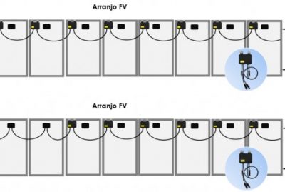
When using optimizers in photovoltaic systems, two types of strings can be formed: complete, in which all modules have optimizers, or selective, in which only some selected modules will receive an optimizer.

Using the optimizer does not eliminate the need for a string inverter. The strings, whether complete or selective, must be connected to the grid-tie inverter in the same way as in any photovoltaic system.

Figura 1: Strings com otimizadores, de forma completa ou seletiva — Figure 1 – Strings with optimizers, completely or selectively

Some optimizer manufacturers require that an inverter of the same brand be used, while other manufacturers allow their optimizers to be compatible with any string inverter available on the market.

In the latter case, where microinverters can be used with inverters from different brands, there is the advantage of eliminating the need to use optimizers in all modules, as long as the string is not in parallel with others on the same inverter MPPT input — that is, only one string per MPPT entry is allowed when there are no optimizers in all modules of the string. This enables selective optimization, providing flexibility to the designer, allowing him to choose where there is a need to optimize.

Furthermore, the possibility of correcting projects even after the start of energy generation is interesting. Optimizers can be added to any existing string, without the need for other system modifications.

IV curves with shading or different orientations

The subject of IV curves in shading situations (without optimizers) was addressed in the article Understanding the effect of partial shadows on photovoltaic systems.

The objective of plotting the IV curve for systems with optimizers is to observe how the inverter's MPPT algorithm will see the string.

In the same way that MPPT searches for the maximum power point (MPP) of a traditional IV curve, it will search for the MPP of another curve that results from the use of optimizers in the string. This way, we can have a more precise view of the effect of using optimizers, identifying where the maximum power points of the string are.

The same reasoning can be used to understand the IV curve of a string with modules in different orientations or slopes.

We will explain the transformation of IV curves in two examples of conventional photovoltaic systems, without the use of optimizers:

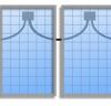
(A) A string with 10 modules (without optimizers) on the same roof, 3 of which are shaded. Conventional photovoltaic system, without optimizers.

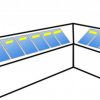
Figura 2 - String do exemplo (A) com três módulos sombreados — Figure 2 – Example string (A) with three shaded modules

(B) A string with 9 modules (without optimizers), 6 for the North and 3 for the East. Conventional photovoltaic system, without optimizers.

Figura 3 - String do exemplo (B) com 6 módulos orientados para o Norte e 3 módulos orientados para o Leste. — Figure 3 – Example string (B) with 6 modules oriented to the North and 3 modules oriented to the East

As IV curves are influenced by irradiance and temperature, they will vary throughout the day. To be able to analyze, we will choose two times of the day: 9:00 am and noon (12:00 pm).

The simulation was carried out using 400 Wp modules, in the city of São Paulo and in January.

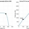
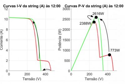
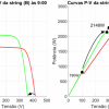
For our example (A), where we have a string of 10 modules, 3 of which are shaded, we have:

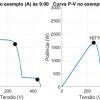
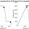
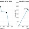
Figura 4 - Curvas I-V e P-V do exemplo (A) às 9:00 horas — Figure 4 – IV and PV curves of example (A) at 9 am

Figura 5 - Curvas I-V e P-V do exemplo (A) às 12h — Figure 5 – IV and PV curves of example (A) at 12h

From the IV curves, the PV curves shown in Figures 4 and 5 are obtained. Note that both PV curves have two peaks. It is very likely that the inverter will operate at the lowest power points (541 W and 773 W) at both times, as the MPPT algorithms existing in string inverters are not capable of differentiating the two peaks existing in each of the PV curves.

As the MPPT algorithm starts tracking from the string's open circuit voltage, at both times the lowest power peaks (541 W and 773 W) are the first to be found, which makes it impossible for the system to reach the points of higher power (1671 W and 2388 W).

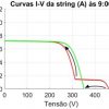
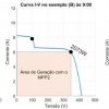
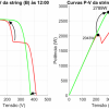
In example (B), in which we have modules in two orientations (North and East) connected in series, we have a similar result:

Figura 6 - Curvas I-V e P-V do exemplo (B) às 9h — Figure 6 – IV and PV curves of example (B) at 9 am

Figura 7 - Curvas I-V e P-V do exemplo (B) às 12h — Figure 7 – IV and PV curves of example (B) at 12h

This time, although we do not have any shading, the PV curves also have two peaks, but this is not as problematic as in the previous case, as the highest power points are further to the right of the curve and will be found by the inverter's MPPT algorithms. .

As in the previous example, a string inverter with traditional MPPT should operate at the peaks on the right: 2073 W at 9:00 am and 2407 W at noon.

Power analysis on curve IV

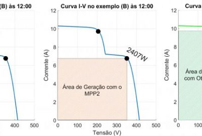
To understand the energy gain of the optimizer, it is important to first understand that we can represent the power generated by the photovoltaic system in curve IV, as shown in Figure 8. The operating power of the inverter is represented by the area of a rectangle formed by the X and Y axes and by the operating point (MPP, maximum power point).

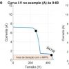
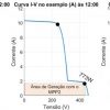
Using the IV curve from example (A) at noon we can illustrate this graphical representation of power:

Figura 8 - Curvas I-V do exemplo (A) às 12h com a área de geração (que representa a potência) destacada em cada ponto de máxima potência (MPP) — Figure 8 – IV curves of example (A) at 12h with the generation area (which represents power) highlighted at each maximum power point (MPP)

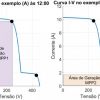
The power generated by operation in MPP1 is equal to the area of the purple rectangle, 9.47 A x 289.3 V = 2739 W. Likewise, the power generated by operation in MPP2 is equal to the area of the red rectangle, 1.87 A x 425.3V = 794W.

Naturally, it is preferable for the inverter to operate at MPP1, but this will not always happen in string inverters without the use of optimizers, as explained previously. Most inverters will make the system operate at MPP2, causing loss of generation.

IV curve with shading and optimizer performance

One of the ways to understand the effect of the optimizer on the photovoltaic module is to imagine that the optimizer is a transformer connected to the module's output. The optimizer manages to increase the module's output current, while reducing its current.

Output power is maintained. Only the voltage and current variables are changed, which makes it possible to make the shaded module compatible with the rest of the string, improving the results of the photovoltaic system.

Figure 9 illustrates the effect of reducing solar irradiance on one of the modules in the set. This module, which would normally have a maximum current of 8 A, now has a short-circuit current of only 6 A. This reduces the maximum power the module can generate.

In the same figure we can see what happens when the optimizer is coupled to the module output: the current range increases to 8 A (compatible with the other modules, which are not shaded) and the voltage range is shortened to less than 40 V .

Optimizers resize the IV curve of these modules, increasing their current and decreasing their voltage. This change is made to the optimizer output. What will be seen by the string inverter is the modified curve, in which the module will be compatible with the rest of the string.

In summary, a module that in a given climatic condition (irradiance and temperature) presents an IV curve with Isc = 6 A and Voc = 48 V, in series with other higher current modules (8 A), will present a resized IV curve.

The module-optimizer set then becomes compatible with higher current modules, delivering an IV curve to the string with Isc = 8A and Voc = 36V, as explained previously.

The result of this is that the lower current modules do not limit the higher current modules and there will not be multiple maximum power points. The string inverter will be able to correctly locate an operating point much higher than what it would find in the system without an optimizer.

Figure 9 - The effect of the optimizer can be observed in the IV curves of a shaded module before and after the optimizer — Figure 9 – The effect of the optimizer can be observed in the IV curves of a shaded module before and after the optimizer

Figure 10 – Transformation of the IV curve before and after the optimizer with the short-circuit current and open-circuit voltage variations highlighted

Now, let's understand what happens to the curves in our examples.

Starting with example (A) at 9:00 hours, the string presents 3 modules with an IV curve of Isc=1.45 A and Voc=46 V, and each optimizer will cause the IV curve to be modified to follow the Isc of the unshaded modules (7.215A).

Figure 11 shows the effect of the optimizer on a shaded module and Figure 12 shows the IV curve resulting from the complete string.

Figure 11 – Transformation of the IV curve of a shaded module in example (A) at 9am

Figura 12 - Transformação da curva I-V da string com atuação dos otimizadores conectados aos três módulos sombreados — Figure 12 – Transformation of the IV curve of the string with the performance of the optimizers connected to the three shaded modules

And the PV curve:

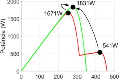
Figura 13 - Transformação da curva P-V da string com atuação dos otimizadores conectados aos três módulos sombreados, destacando-se o novo ponto de máxima potência (1831 W) — Figure 13 – Transformation of the PV curve of the string with the performance of the optimizers connected to the three shaded modules, highlighting the new point of maximum power (1831 W)

It is interesting to note how optimizers make the work of the string inverter's MPPT easier, making it “see” only one peak. And at this point of operation, each module is generating its maximum individually.

Doing the power analysis, we have:

Figura 14 - Área de geração no exemplo (A) às 9-00 horas para- MPP1 (1671 W) e MPP2 (541 W) para a string sem otimizadores; e MPP (1831 W) para a string com otimizadores — Figure 14 – Generation area in example (A) at 9-00 hours for- MPP1 (1671 W) and MPP2 (541 W) for the string without optimizers; and MPP (1831 W) for the string with optimizers

We note that with the use of optimizers the power generated is greater than the powers generated in any of the previous peaks. Instead of generating 1,671 W or 541 W, the system manages to generate 1831 W. In other words, the result with the optimizer is higher than what would be obtained even if the string inverter was able to locate MPP1.

The same methodology was applied to the other examples. For each one, the IV and PV curves were generated for the string without optimizers and with optimizers, and the generation areas in the IV curves for the string without optimizers and with optimizers.

For example (A), with 3 modules shaded at noon:

Figura 15 - Transformação das curvas I-V e P-V, no exemplo (A) às 12h, da string com atuação dos otimizadores conectados aos três módulos sombreados, destacando o novo ponto de máxima potência (2616 W) — Figure 15 – Transformation of the IV and PV curves, in example (A) at 12h, of the string with the performance of the optimizers connected to the three shaded modules, highlighting the new point of maximum power (2616 W)

Figura 16 - Área de geração no exemplo (A) às 12h para- MPP1 (2388 W) e MPP2 (773 W) para a string sem otimizadores; e MPP (2616 W) para a string com otimizadores — Figure 16 – Generation area in example (A) at 12h for- MPP1 (2388 W) and MPP2 (773 W) for the string without optimizers; and MPP (2616 W) for the string with optimizers

For example (B) of a string with modules in two orientations at 9:00 am, when the irradiance on the East roof is greater than the irradiance on the North roof:

Figura 17 - Transformação das curvas I-V e P-V, no exemplo (B) às 9h, da string com atuação dos otimizadores conectados aos módulos ao Norte destacando o novo ponto de máxima potência (2148 W) — Figure 17 – Transformation of the IV and PV curves, in example (B) at 9am, of the string with the performance of the optimizers connected to the modules to the North, highlighting the new point of maximum power (2148 W)

Figura 18 - Área de geração no exemplo (B) às 9h para- MPP1 (790 W) e MPP2 (2073 W) para a string sem otimizadores; e MPP (2148 W) para a string com otimizadores — Figure 18 – Generation area in example (B) at 9am for- MPP1 (790 W) and MPP2 (2073 W) for the string without optimizers; and MPP (2148 W) for the string with optimizers

For example (B) at noon when the irradiance received by the modules to the North is higher than the irradiance received by the modules to the East:

Figura 19 - Transformação das curvas I-V e P-V, no exemplo (B) às 12h, da string com atuação dos otimizadores conectados nos módulos Leste destacando o novo ponto de máxima potência (2789 W) — Figure 19 – Transformation of the IV and PV curves, in example (B) at 12h, of the string with the performance of the optimizers connected to the East modules highlighting the new maximum power point (2789 W)

Figura 20 - Áreas de geração no exemplo (B) às 12h para- MPP1 (2043 W) e MPP2 (2407 W) para a string sem otimizadores; e MPP (2789 W) para a string com otimizadores — Figure 20 – Generation areas in example (B) at 12h for- MPP1 (2043 W) and MPP2 (2407 W) for the string without optimizers; and MPP (2789 W) for the string with optimizers

Conclusion

The use of optimizers provides flexibility to the designer, increasing their possibilities regarding the configuration of photovoltaic systems and increasing the maximum power that can be extracted from photovoltaic strings in adverse conditions (shading, different module orientations).

With power optimizers used integrally or selectively (only on problematic modules), a range of possibilities opens up, such as:

extend old strings with modules of different powers;
connect modules from small roofs in series with modules from other roofs;
employ inverters with a smaller number of MPPT inputs;
use the same MPPT in more than one orientation or inclination or maximize the use of the customer's roof by connecting modules in areas that suffer from shadows.

The characteristic curves “seen” by the inverter show how the optimizer technology for string inverters works. Tracking the point of maximum power by the MPPT algorithm is facilitated and this technology guarantees maximum efficiency of the photovoltaic system.

Hugo Soeiro Moreira

Technical manager at Tigo Energy LATAM. Specialist in photovoltaic systems. PhD student and master in electrical engineering from UNICAMP. Dedicated to studying the topics: Module shading, MPPT techniques, and Power optimizers for photovoltaic generation systems. He is a researcher at the Energy and Photovoltaic Systems Laboratory and the Power Electronics Laboratory (LEPO) at UNICAMP.