
At the end of 2021, at Intersolar South America, Electro Graphics presented one of its new features for SOLergo 2022, the possibility of developing a 3D layout in photovoltaic projects.
From this, software users will be able to carry out 3D modeling of the project installation location, calculation of losses due to shading, and also the arrangement of photovoltaic modules.
This tutorial will show you how to use the new 3D layout for SOLergo 2022.
Tutorial
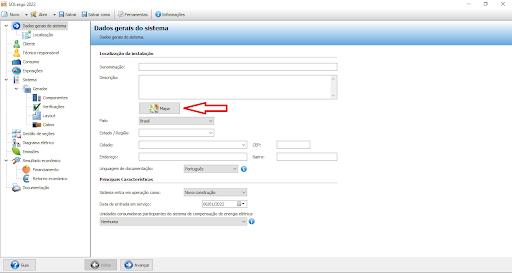
To use the SOLergo 3D Layout tool, you will first need to define the location of the photovoltaic project. To do this, the first step will be to click on the “Map” icon, located in the “General system data” window, as shown in Figure 1.
After clicking on the “Map” icon, the software will open another reduced Google Maps window, making it possible to choose the location in two ways, the first way is to enter the address in the first field of the window, and the second way is to select the location directly on the map, as shown in Figure 2.
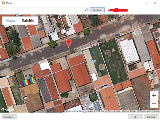
To carry out the PV project, the address was defined on a street located in the city of Hortolândia/SP, as shown in Figure 2, and after that, to continue building the 3D layout, access the “Exhibitions” window and select the “Installation Type” in the “Orientation” field, as shown in Figure 3.
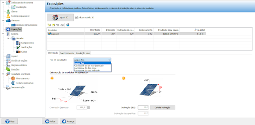
As the project in question is residential, the type was selected as “Fixed angle” since the PV modules will be fixed to the roof. Once this is done, the next step consists of building the project in 3D, by clicking on the “3D Layout” icon Still in the “Exhibitions” window, a new window will open where it will be possible to import the planimetry, as shown in Figure 4.
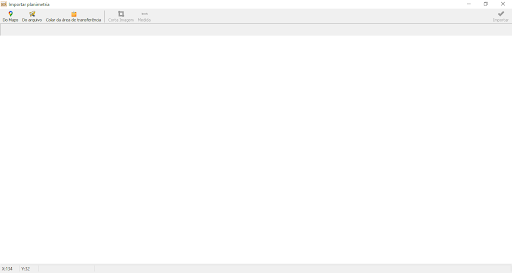
Importing planimetry can be carried out in two ways, the first way is via Google Maps, clicking on the “Do Maps” icon will open a window identical to that in Figure 2, the second way is by importing a 360° photo directly from the computer, by clicking on the “From file” icon, both shown in Figure 4.
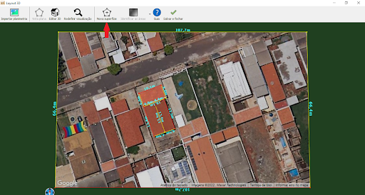
For this article, the method chosen was to use planimetry imported via Google Maps. Therefore, after choosing the residence, see Figure 2, it is necessary to define the surfaces of the residence, create surfaces for each area of the chosen land and for each roof water.


As the chosen residence has a garage and the roof of the house has gables, it will be necessary to create three surfaces. For each surface to be created, it will be necessary to click on the “New surface” icon and define the contours of the area, as shown in Figure 5.
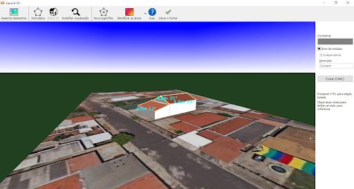
After creating the surfaces of the residence, construction of the 3D layout begins. By clicking on the “Edit 3D” icon, you can configure the height and inclination of the residence. To configure the height of the surface, click and hold on the circle located at the end of the reference edge (red), and move the cursor according to the desired height.
To configure the surface inclination, the process is similar, differing only in the edge, which for the inclination configuration will be yellow. To edit each surface separately, you must press and hold the “Control” button on the keyboard before carrying out the process described previously.
Still in the 3D layout editing part, it is possible to identify independent surfaces and also define which surface will be an area for module allocation, as shown in Figure 6.
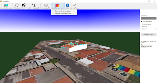
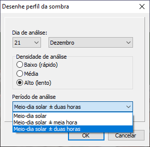
The next step in the construction of the 3D layout will be the identification of the shadow profiles, for this, when clicking on the “Identify areas” icon, the option “trace shadow profiles…” was selected, as Figure 7 shows, and this will appear a new window for configuring the shadow profile, allowing the day, density and analysis time to be configured, as shown in Figure 8.
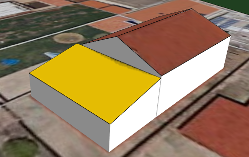
Then, with the shadow profile drawn, the layout shows the shading arrangement in the area where the photovoltaic modules will be allocated. For this project, the modules will be allocated to the garage roof, as Figure 9 shows.
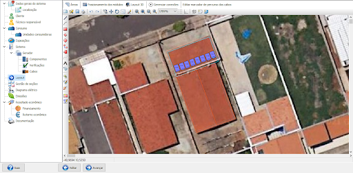
When finishing the “Exhibitions” section, it will be possible to allocate the modules in the constructed layout. As a result, the 2D design for allocating the modules will appear in the “Layout” window. This allocation can be done automatically by the software, but there is also the possibility of configuring the arrangement of modules manually. For this project, 8 300Wp PV modules were used in series for 1 inverter with MPPT, as shown in Figure 10.
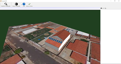
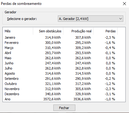
Based on this, it becomes possible to visualize the project in 3D with the PV modules located on the roof. When clicking on the “3D Layout” icon within the “Layout” window, a new tab opens with the finished 3D layout, as shown in Figure 11. Furthermore, in this same icon in Figure 11 it is possible to quantify the loss values due to shading. When clicking on the “Start simulation” icon, a new tab will open with the monthly values and the annual value of losses due to shading.